From Noise to Structure: Diffusion Models and Flow Matching

Abstract

This project investigates diffusion-based generative models through both pretrained applications and training from scratch. First, a pretrained model (DeepFloyd IF) is used for text-to-image generation, denoising, image editing, and visual anagram synthesis, demonstrating the impact of iterative denoising and classifier-free guidance (CFG) on image quality. Second, models are trained on MNIST to study the fundamentals of generative learning. A one-step denoising UNet is shown to collapse under an MSE objective when inputs contain no informative structure, producing averaged outputs. To address this, a flow matching model is implemented, learning a continuous transformation from noise to data via time conditioning. The model is further extended with class conditioning and CFG, enabling controlled and higher-quality generation. Overall, the results highlight the limitations of naive denoising and demonstrate the effectiveness of flow-based approaches for stable and controllable image generation.

Part 1: Power of Diffusion Models

In this section, a pretrained diffusion model (DeepFloyd IF) is utilized to perform various image generation and processing tasks without any fine-tuning.

1.1 DeepFloyd IF — Pretrained Diffusion Model

DeepFloyd IF is a two-stage text-to-image diffusion model developed by Stability AI. The first stage generates images at 64×64 resolution, while the second stage upsamples these outputs to 256×256. Since the model cannot directly accept raw text strings, prompts must first be encoded into embeddings — high-dimensional vectors (4096-dimensional in this case) that the model can process. A HuggingFace pipeline is used to convert text prompts into embeddings, which are saved as .pth files and passed as input to DeepFloyd IF.

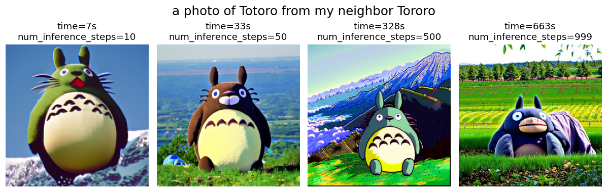
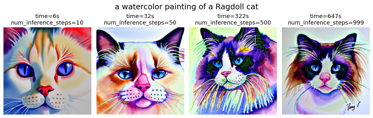
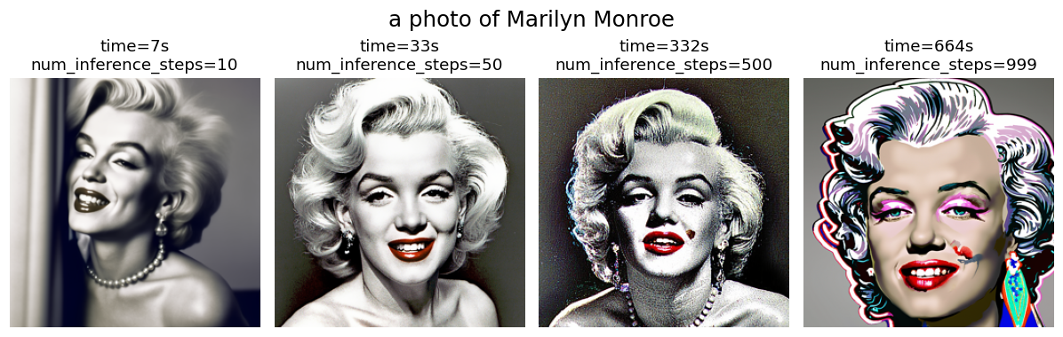
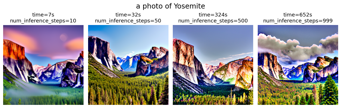
Figure 1 shows images generated from text prompts with varying numbers of inference steps (num_inference_steps) and their corresponding execution times. Since the model is trained over 1000 discrete timesteps, the maximum value of num_inference_steps used here is 999. As expected, a low step count yields images of noticeably lower quality. Increasing num_inference_steps progressively adds finer details and textures to the output, but also increases execution time linearly. Beyond 500 steps, the execution time is doubled while the improvement in visual quality becomes marginal.

1.2 Diffusion Model Denoising

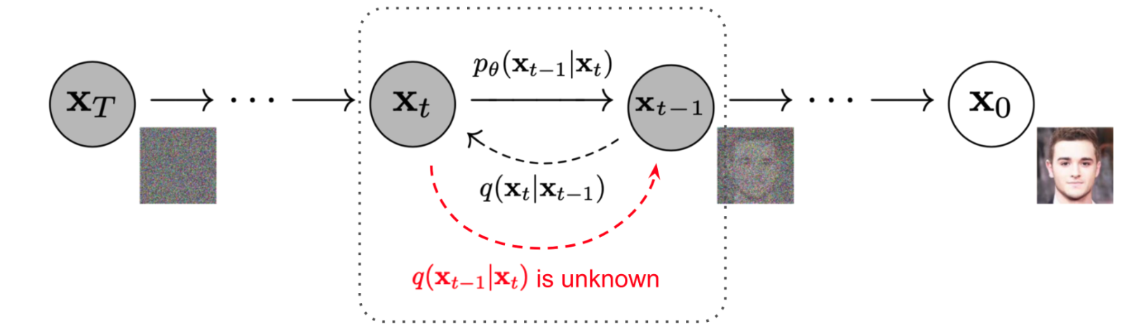
Starting from a clean image \(x_0\), noise is iteratively added to produce progressively noisier versions \(x_t\), until pure noise is reached at timestep \(t = T\) (\(T=1000\) in this study). A diffusion model learns to reverse this process, as shown in Figure 2. Given a noisy image \(x_t\) and the timestep \(t\), the model predicts the noise present in the image. Using this prediction, the noise can either be fully removed to obtain a direct estimate of \(x_0\), or partially removed to obtain an estimate of \(x_{t-1}\) with slightly less noise.

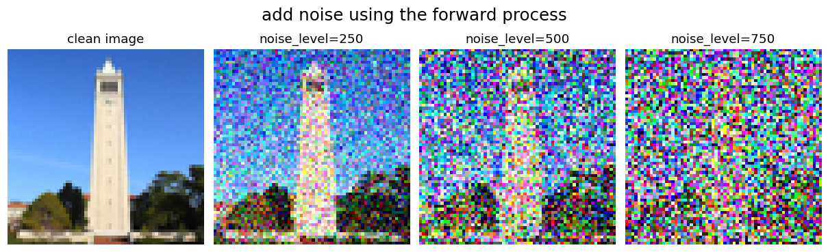
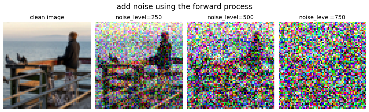
1.2.1 The Forward Process

The forward process corrupts a clean image by progressively adding Gaussian noise, as defined by:

which is equivalent to computing: That is, given a clean image \(x_0\), we get a noisy image \(x_t\) at timestep \(t\) by sampling from a Gaussian with mean \( \sqrt{\bar{\alpha_t}}x_0 \) and variance \( (1-\bar{\alpha_t}) \). The \(\bar\alpha_t\) is from the pretrained diffusion model variable alphas_cumprod. Note that \(t=0\) corresponds to a clean image and larger \(t\) corresponds to more noise; consequently, \(\bar{\alpha}_t\) approaches 1 for small \(t\) and 0 for large \(t\).

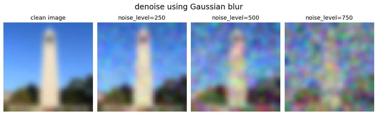
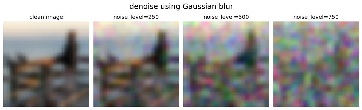
1.2.2 Classical Denoising: Gaussian Blur Baseline

Gaussian blur is a classical image smoothing technique that convolves the image with a Gaussian kernel, replacing each pixel with a weighted average of its neighbors. The standard deviation \(\sigma\) controls the blur strength — a larger \(\sigma\) removes more noise but also loses more detail. It is applied here as a simple baseline for comparison against the diffusion-based denoiser, using sigma = 2 and kernel_size = 13 to cover over 99% of the Gaussian density.

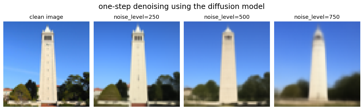
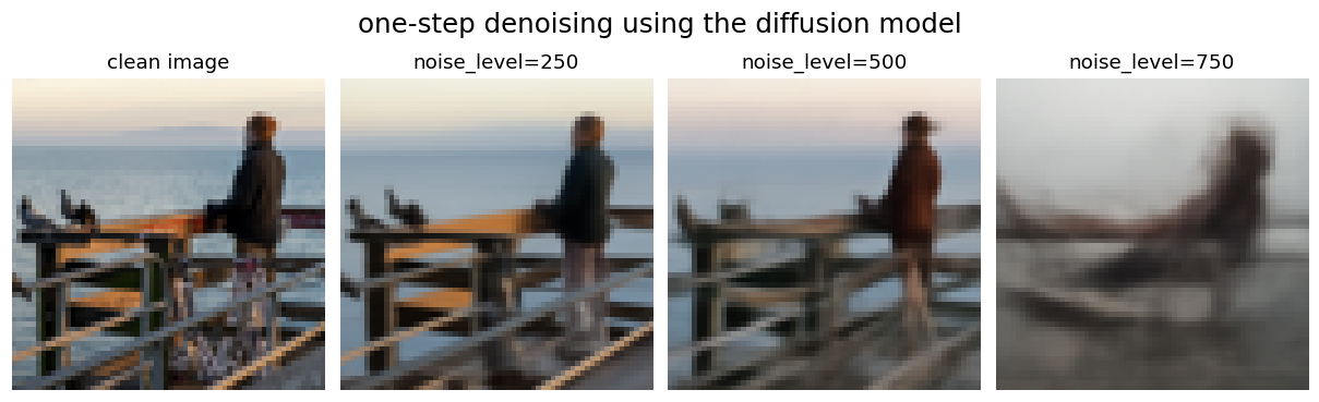
1.2.3 One-step Denoising Using the Diffusion Model

The denoiser of the pretrained DeepFloyd model is accessible via stage_1.unet, a UNet trained on a large dataset of \((x_0, x_t)\) image pairs. The UNet is conditioned on the noise level by taking the timestep \(t\) as an additional input. Since the model was trained with text conditioning, a neutral prompt embedding ("a high quality photo") is used. The one-step denoising procedure is as follows: first, Gaussian noise is added to the clean image at a given timestep \(t\); the noisy image, timestep, and prompt embedding are then passed to stage_1.unet to estimate the noise; finally, the estimated noise is subtracted to recover a clean estimate of \(x_0\).

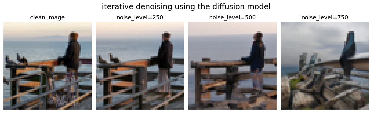
1.2.4 Iterative Denoising Using the Diffusion Model

Unlike one-step denoising, diffusion models are designed to denoise iteratively. In principle, one could start from pure noise \(x_T\) at timestep \(T = 1000\), denoise one step at a time to obtain \(x_{999}, x_{998}, \ldots\), and continue until reaching \(x_0\). However, this requires running the UNet 1000 times, which is computationally expensive. In practice, inference can be accelerated by skipping timesteps — a technique justified by the connection between diffusion models and differential equations, which allows larger steps without significant loss in quality.

To skip steps, a reduced list of timesteps strided_timesteps is constructed, much shorter than the full 1000-step sequence. strided_timesteps[0] corresponds to the largest \(t\) (the noisiest image) and strided_timesteps[-1] corresponds to \(t = 0\) (the clean image). A uniform stride of 30 works well in practice.

At the \(i\)-th denoising step, the current timestep is \(t = \)strided_timesteps[i] and the target is \(t' = \)strided_timesteps[i+1], stepping from noisier to cleaner. The transition is given by:

where:

• \(x_t\) — the image at timestep \(t\)
• \(x_{t'}\) — the image at timestep \(t' < t\) (less noisy)
• \(\bar{\alpha}_t\) — defined by alphas_cumprod, as described above
• \(\alpha_t = \bar{\alpha}_t / \bar{\alpha}_{t'}\)
• \(\beta_t = 1 - \alpha_t\)
• \(x_0\) — the current clean image estimate, obtained as in the previous section

The term \(v_\sigma\) is a predicted noise variance term. In DeepFloyd, this is predicted by the model itself and added via the supplied add_variance function.

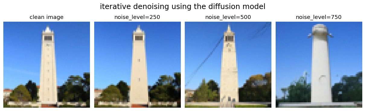
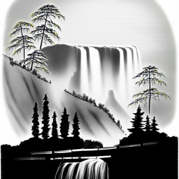
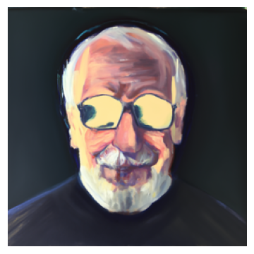
1.2.5 Denoising Results

Two 64×64 images — Sather Tower and an old man facing the sea — are used to evaluate the denoising methods, as shown in Figures 3 and 4. Each clean image is first corrupted using the forward process at noise levels (timesteps) of 250, 500, and 750, then denoised using three methods: Gaussian blur, one-step diffusion denoising, and iterative diffusion denoising (top to bottom in the figures).

Gaussian blur performs poorly at recovering image content. Because the forward process removes fine structural details, and Gaussian blur only smooths pixel values, it cannot reconstruct high-frequency structures. The diffusion model, by contrast, recovers these details effectively. At low to moderate noise levels, the one-step denoiser restores plausible images with sharp details. However, at high noise levels (e.g., timestep 750), too much information is lost and the model begins to hallucinate content inconsistent with the original.

Iterative denoising further improves reconstruction quality at lower noise levels, producing sharper and more detailed results than one-step denoising at timesteps 250 and 500. However, it also tends to hallucinate more at higher noise levels. For example, in Figure 3 at timestep 750, the reconstructed image no longer resembles a tower, and in Figure 4 at timestep 500, the clothing and hat of the old man differ noticeably from the original.

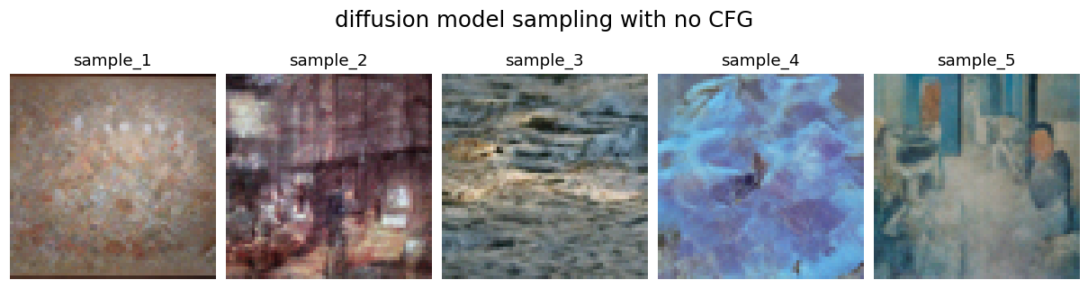
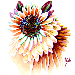
1.3 Image Generation via Iterative Sampling

Beyond image denoising, the iterative denoising function can also be used to generate images from scratch. Instead of starting from a partially noisy image, passing pure noise as input allows the model to synthesize a completely new image. Figure 5 shows five samples generated this way. While the results are visually coherent, the image quality is limited — fine details and structures are often missing without additional guidance.

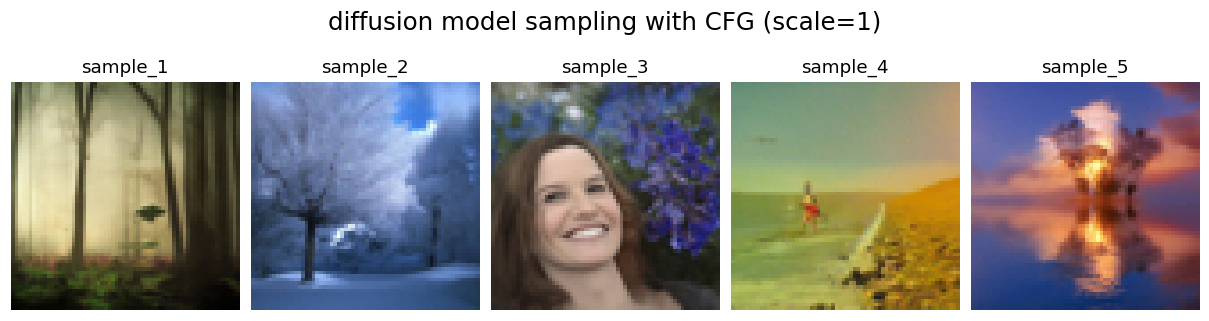
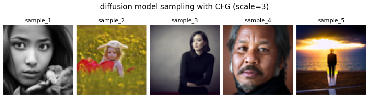
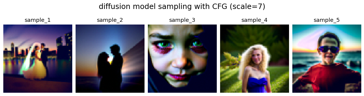
To improve image quality at the expense of diversity, Classifier-Free Guidance (CFG) was applied. Two noise estimates were computed: a conditional estimate \(\epsilon_c\) based on a text prompt, and an unconditional estimate \(\epsilon_u\). The final noise estimate is then:

where \(\gamma\) is a scale parameter controlling the guidance strength. When \(\gamma = 0\), the estimate is fully unconditional; when \(\gamma = 1\), it is fully conditional. For \(\gamma > 1\), the model produces noticeably sharper and higher-quality images, though the theoretical explanation for this behaviour remains an open question. Figure 6 shows samples generated with CFG at different values of scale. Compared with Figure 5, the results contain significantly more detail and structure. As scale increases, the images become progressively sharper, but at scale = 7 the outputs begin to appear over-sharpened and unnatural.

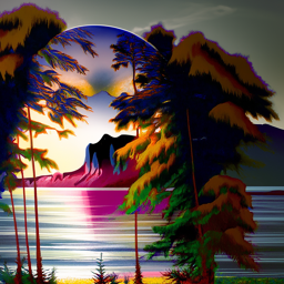
1.4 Image-to-Image Translation

Beyond denoising, diffusion models can also be applied to image editing. As discussed in Section 1.2, adding noise to a clean image and denoising it causes the model to synthesize new content, effectively projecting the noisy image back onto the manifold of natural images. Image editing exploits this property: by controlling the amount of noise added, one can control the degree of modification. The experiments in this section follow the SDEdit algorithm.

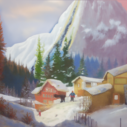
1.4.1 Image Editing

Several clean images were noised at different levels and then denoised without text conditioning, as shown in Figure 7. The parameter i_start controls the noise level: a lower value corresponds to more noise added. At high i_start values (low noise), the output remains visually close to the original while the model enriches it with finer details, improving overall quality. Notably, it can even translate 2D cartoon images into photorealistic 3D renderings (e.g., the avocado image). As i_start decreases and more noise is added, the output progressively deviates from the source. Below i_start = 10, the generated images bear little resemblance to the original.

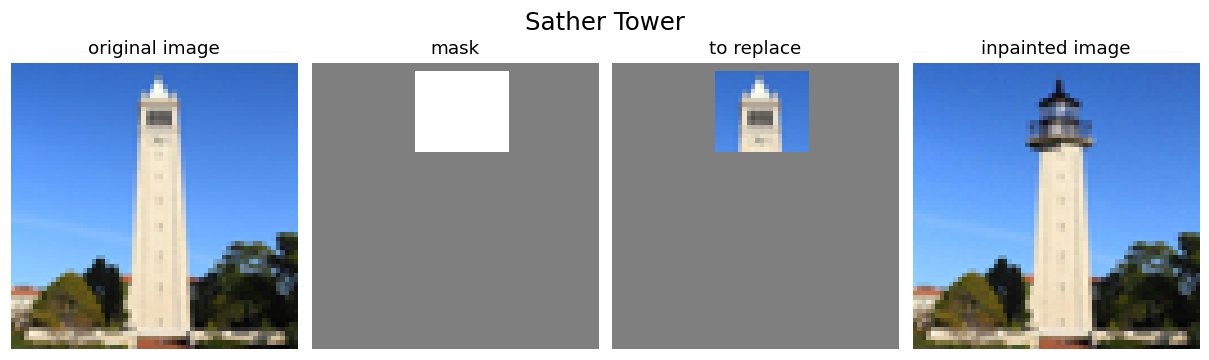
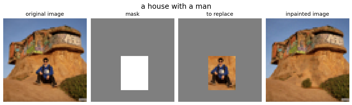
1.4.2 Image Inpainting

The same procedure was extended to image inpainting, following the RePaint algorithm. Given an original image \(x_\text{orig}\) and a binary mask \(\mathbf{m}\), the goal is to generate a new image that preserves the original content wherever \(\mathbf{m} = 0\) and synthesizes new content wherever \(\mathbf{m} = 1\). This is achieved by running the standard denoising loop with one modification: at each timestep, after obtaining \(x_t\), the unmasked region is replaced with the correspondingly noised version of the original image:

This ensures that pixels outside the mask remain consistent with \(x_\text{orig}\) at the appropriate noise level for timestep \(t\), while pixels inside the mask are generated freely by the diffusion model.

Figure 8 shows two images inpainted using the RePaint algorithm without text prompts. In the first example, a mask covers the upper portion of Sather Tower, which the model replaces with the structure of a lighthouse top. In the second, a mask covers the man in front of a house, and the model fills the region with natural ground that blends seamlessly with the surroundings. Both results demonstrate effective and coherent inpainting.

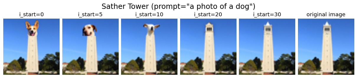
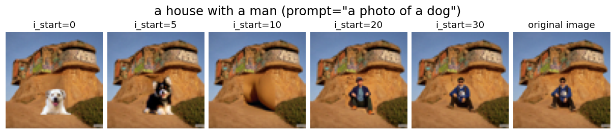
1.4.3 Text-Conditioned Image-to-Image Translation

The same inpainting procedure was applied with a descriptive text prompt — "a photo of a dog" in this case — to steer the synthesized content toward a specific target, as shown in Figure 9. The effect of noise level was examined by varying i_start. At low noise levels, the output remains close to the original with only minor detail changes, and the prompt has little visible influence. As the noise level increases (i.e., lower i_start), the prompt-driven features become apparent: the top of Sather Tower is replaced by a dog's head, and the man in front of the house is replaced by a dog. In both cases, the inpainted regions blend naturally with the surrounding image, demonstrating the effectiveness of diffusion-based image editing.

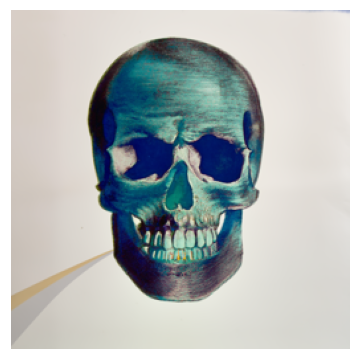
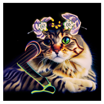
1.5 Visual Anagrams

Visual anagrams are optical illusions generated by diffusion models that reveal different content depending on viewing orientation or distance. The key idea is to combine noise estimates computed under different conditions at each denoising step, so that the image satisfies two prompts simultaneously. Three variants are explored below: flip anagrams, frequency-based anagrams, and negative anagrams.

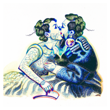
1.5.1 Flip Anagrams

In flip anagrams, \(x_t\) is denoised with prompt \(p_1\) to obtain \(\epsilon_1\). Simultaneously, \(x_t\) is rotated 180° and denoised with prompt \(p_2\) to obtain \(\epsilon_2\), which is then rotated back. The two estimates are averaged to form the final noise estimate for the reverse step:

where \(\text{flip}(\cdot)\) denotes a 180° rotation and \(p_1\), \(p_2\) are two different text prompt embeddings. Figure 10 shows the generated images — each can be interpreted as a distinct scene depending on viewing orientation.

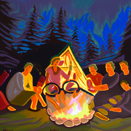
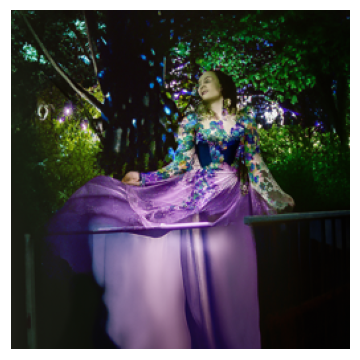
1.5.2 Frequency Anagrams

Frequency-based hybrid images are generated following a similar approach to the flip anagram technique. A composite noise estimate \(\epsilon\) is constructed by computing noise estimates under two different text prompts and combining their frequency components: low frequencies from \(\epsilon_1\) and high frequencies from \(\epsilon_2\). The algorithm is:

where \(f_\text{lowpass}\) and \(f_\text{highpass}\) are low-pass and high-pass filters (implemented as Gaussian blur with kernel size 33 and \(\sigma = 2\)), and \(p_1\), \(p_2\) are two different text prompt embeddings. The resulting image appears as one scene up close and a different scene when viewed from a distance, as shown in Figure 11.

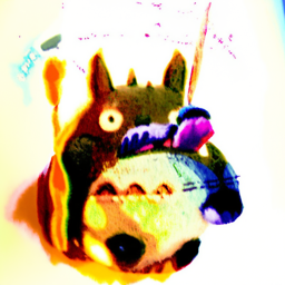
1.5.3 Negative Anagrams

Negative anagrams follow an analogous approach to flip anagrams, but instead of rotating the image, the color-inverted image \(-x_t\) is used. Specifically, \(x_t\) is denoised with prompt \(p_1\) to obtain \(\epsilon_1\). Simultaneously, the color-inverted image \(-x_t\) is denoised with prompt \(p_2\), and the resulting estimate is negated to obtain \(\epsilon_2\). The two are then averaged to form the final noise estimate:

where \(p_1\) and \(p_2\) are two different text prompt embeddings. Figure 12 shows the generated negative anagrams, animated to illustrate how the perceived content changes upon color inversion.

Part 2: Flow Matching from Scratch

Unlike the previous section, which relied on a pretrained model, this section trains flow matching models from scratch. The MNIST dataset is used for its simplicity and accessibility. MNIST is a widely used benchmark consisting of 70,000 grayscale images of handwritten digits (0–9), each 28×28 pixels in size, split into 60,000 training and 10,000 test samples. Its small image size and well-understood structure make it an ideal testbed for training and evaluating generative models.

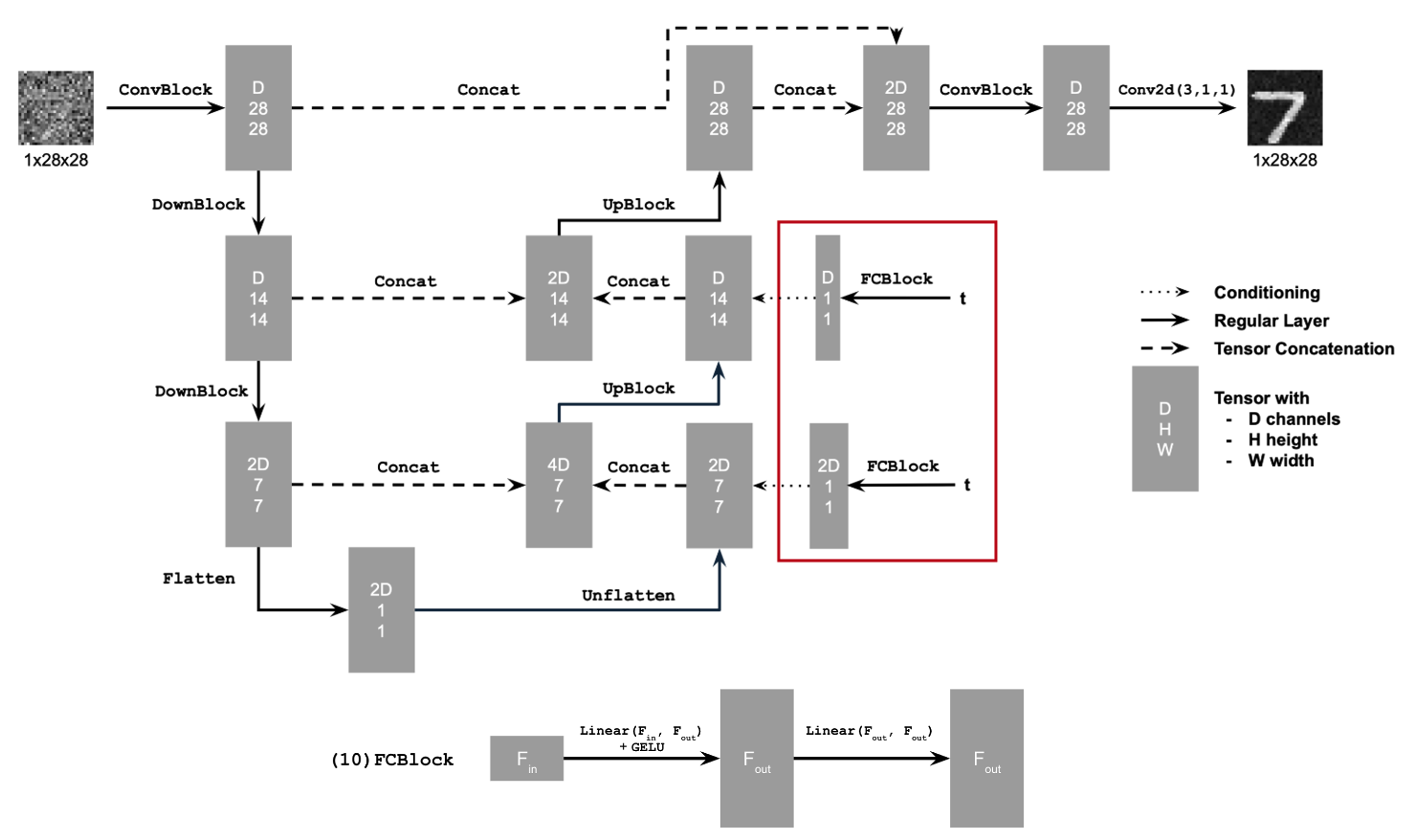
2.1 Single-Step Denoising UNet

A UNet is trained as a one-step denoiser \(D_\theta\), which maps a noisy image \(z\) to a clean image \(x\). It is optimized over an L2 loss:

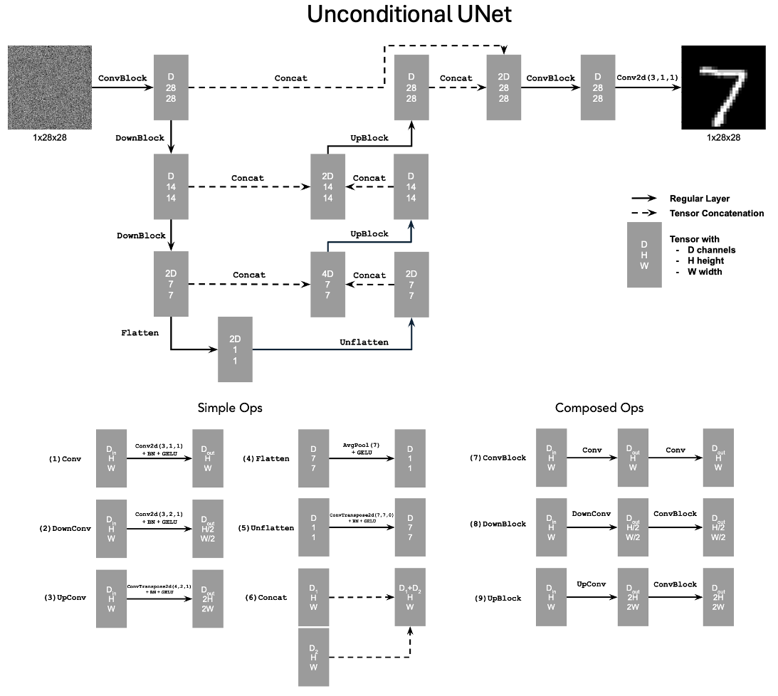
The UNet consists of downsampling, upsampling, and flatten/unflatten blocks with skip connections, as illustrated in Figure 13.

• Conv2d(kernel_size, stride, padding) is nn.Conv2d()
• BN is nn.BatchNorm2d()
• GELU is nn.GELU()
• ConvTranspose2d(kernel_size, stride, padding) is nn.ConvTranspose2d()
• AvgPool(kernel_size) is nn.AvgPool2d()
• D is the number of hidden channels and is a hyperparameter set during training.

At a high level, the blocks do the following:

• (1) Conv is a convolutional layer that doesn't change the image resolution, only the channel dimension.
• (2) DownConv is a convolutional layer that downsamples the tensor by 2.
• (3) UpConv is a convolutional layer that upsamples the tensor by 2.
• (4) Flatten is an average pooling layer that flattens a 7x7 tensor into a 1x1 tensor. 7 is the resulting height and width after the downsampling operations.
• (5) Unflatten is a convolutional layer that unflattens/upsamples a 1x1 tensor into a 7x7 tensor.
• (6) Concat is a channel-wise concatenation between tensors with the same 2D shape. This is simply torch.cat().

Composed operations are built from simple operations in order to make the network deeper. This doesn't change the tensor's height, width, or number of channels, but simply adds more learnable parameters.

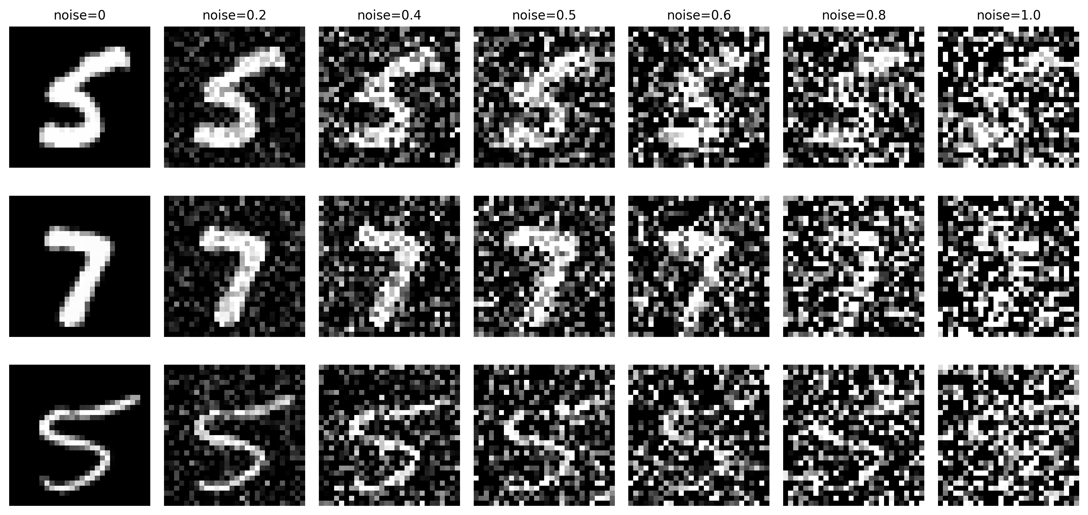
2.1.1 Noising MNIST Digits

To train the denoiser, data pairs \((z, x)\) are constructed by corrupting clean MNIST digits \(x\) with Gaussian noise according to the following process:

Figure 14 visualizes the effect of different noise levels \(\sigma = [0.0, 0.2, 0.4, 0.5, 0.6, 0.8, 1.0]\) on normalized inputs \(x \in [0, 1]\). As expected, image quality degrades progressively with increasing \(\sigma\).

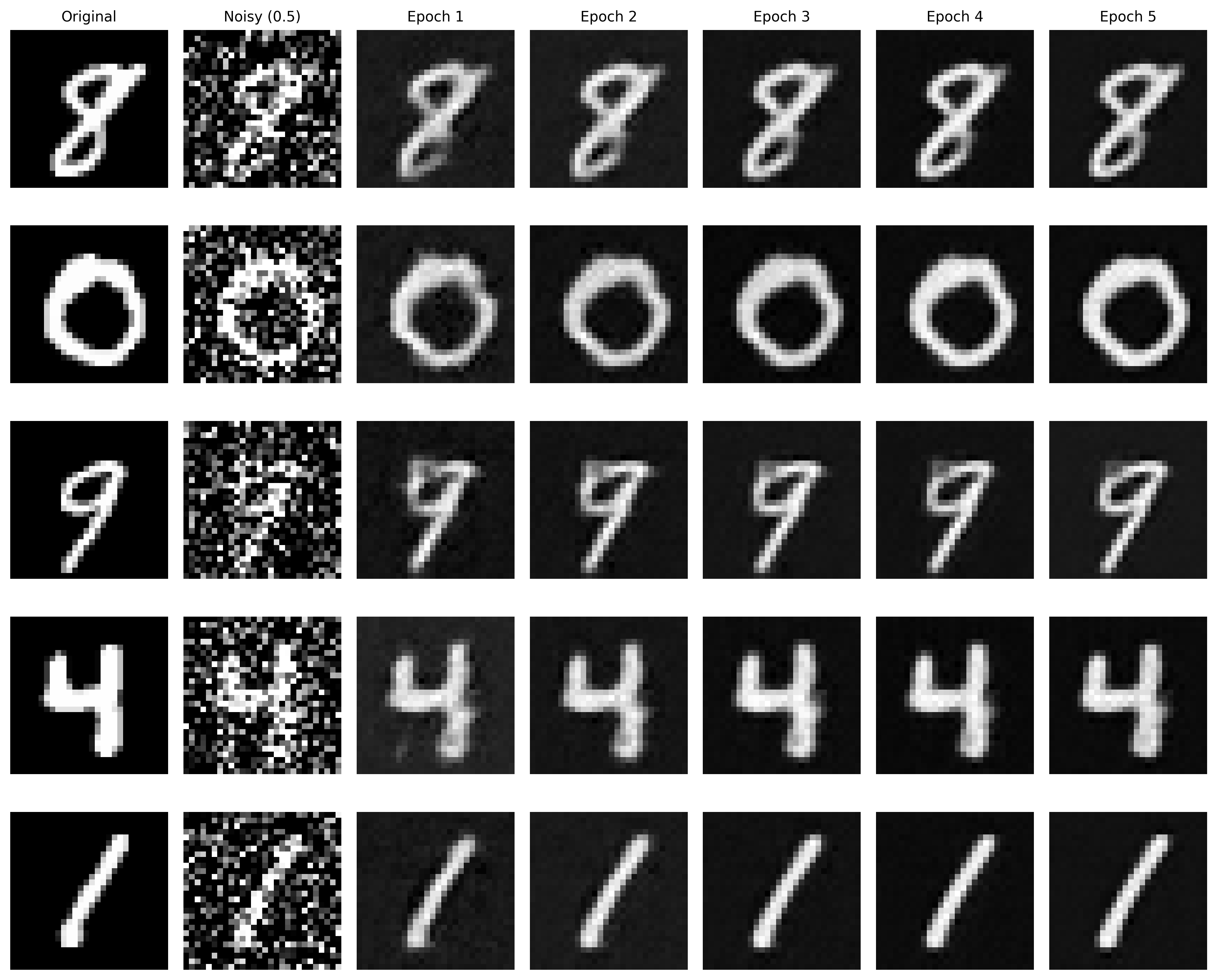
2.1.2 Training

The denoiser was trained to recover clean images \(x\) from noisy inputs \(z\) at a fixed noise level of \(\sigma = 0.5\). The MNIST training split was loaded via torchvision.datasets.MNIST with shuffling enabled and a batch size of 256. Noise was applied on-the-fly at each batch fetch, ensuring the network saw a fresh random \(\epsilon\) at every iteration and improving generalization. The UNet from Section 2.1 was used with hidden dimension D = 128 and optimized with Adam at a learning rate of 1e-4 for 5 epochs. Denoised results on the test set were recorded after the 1st and 5th epoch to track reconstruction quality over training. 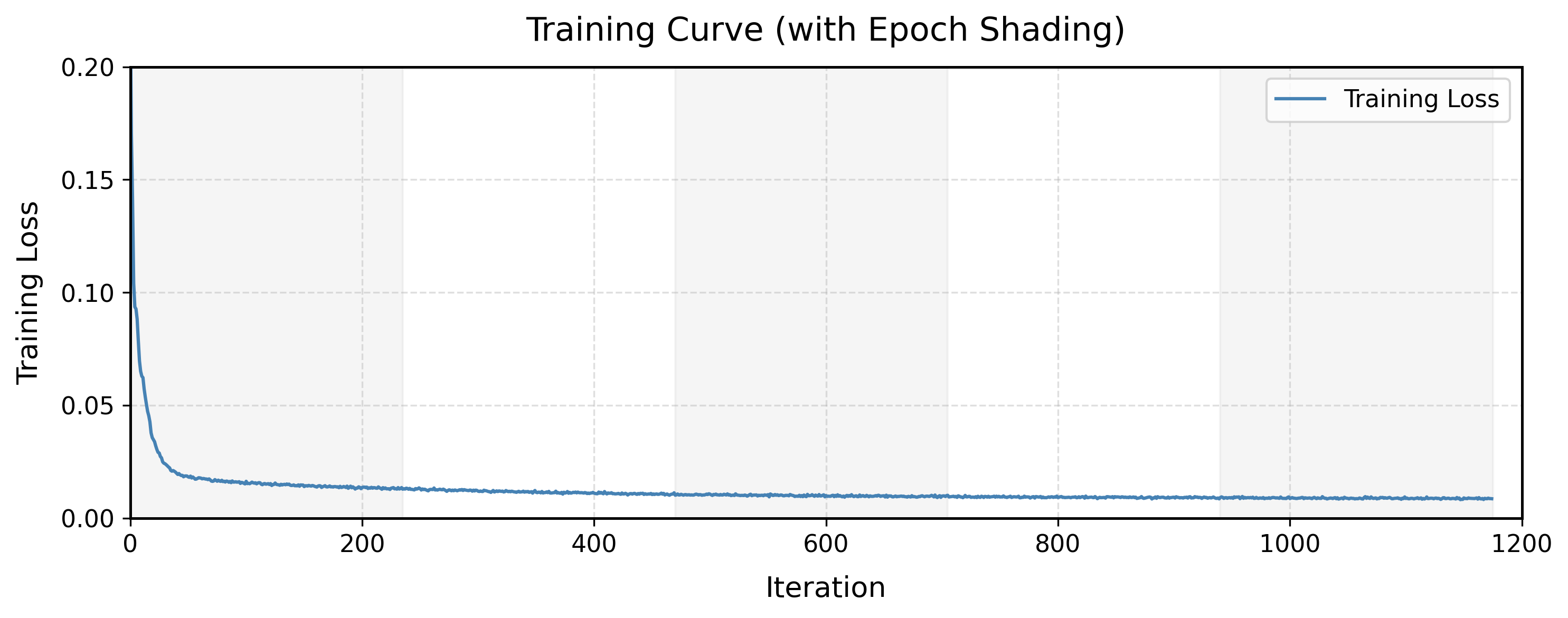Figures 15 and 16 show the training loss curve and denoised outputs at each epoch, respectively. The model converges rapidly within the first 50 iterations; beyond that, the loss continues to decrease but at a much slower rate. This trend is consistent with the visual results: after epoch 1 the denoised images are already recognizable, and the improvement in image quality from epoch 2 to epoch 5 is marginal.

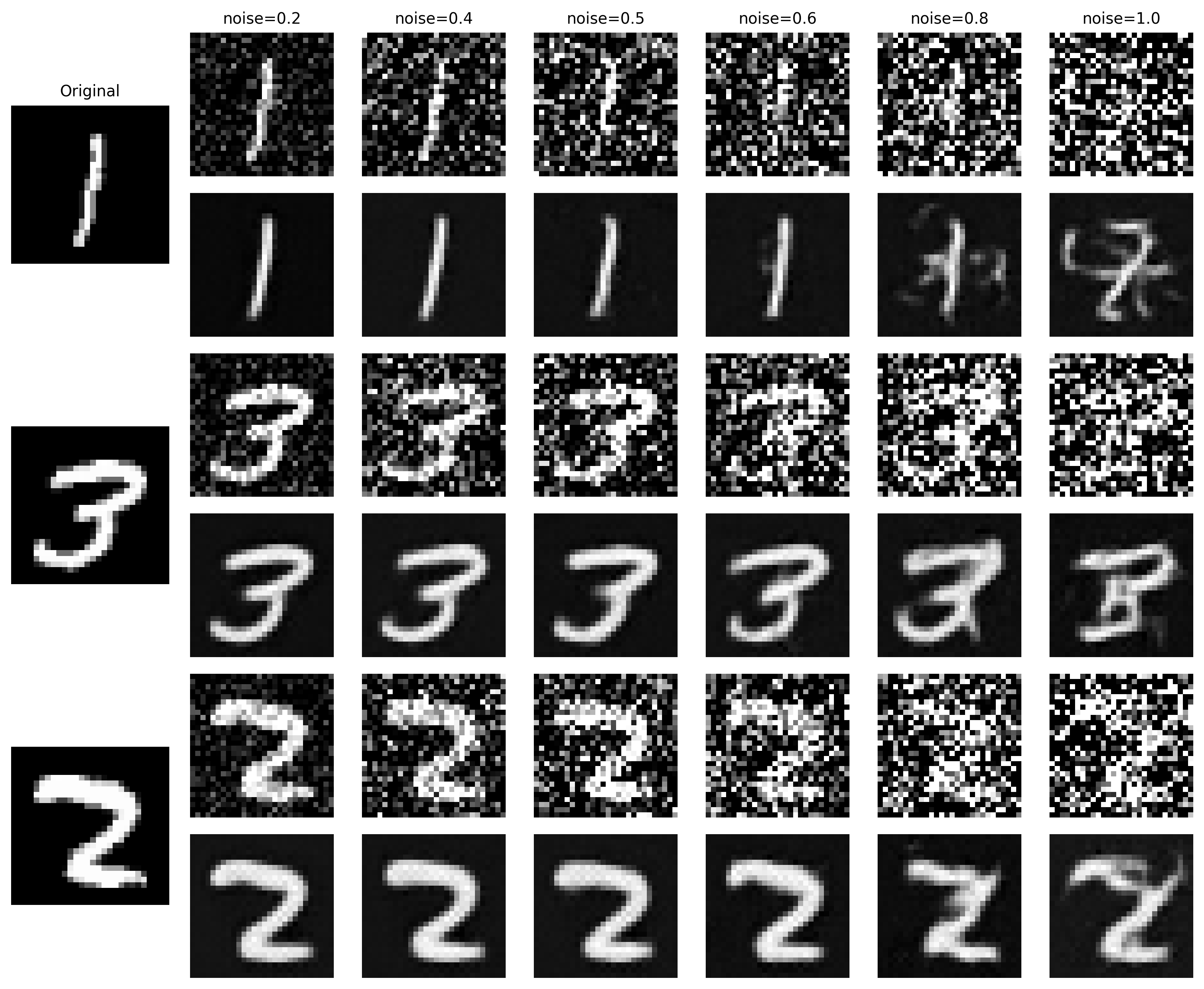
2.1.3 Out-of-Distribution Testing

Since the denoiser was trained exclusively at \(\sigma = 0.5\), it was evaluated on MNIST digits corrupted at out-of-distribution noise levels \(\sigma \in \{0.2, 0.4, 0.5, 0.6, 0.8, 1.0\}\) to assess generalization, as shown in Figure 17. The denoiser performs well for noise levels up to 0.6, producing clean and recognizable reconstructions. At \(\sigma = 0.8\) and \(\sigma = 1.0\), however, the outputs deteriorate significantly and are largely unrecognizable. This is expected, as the model was never exposed to such high noise levels during training.

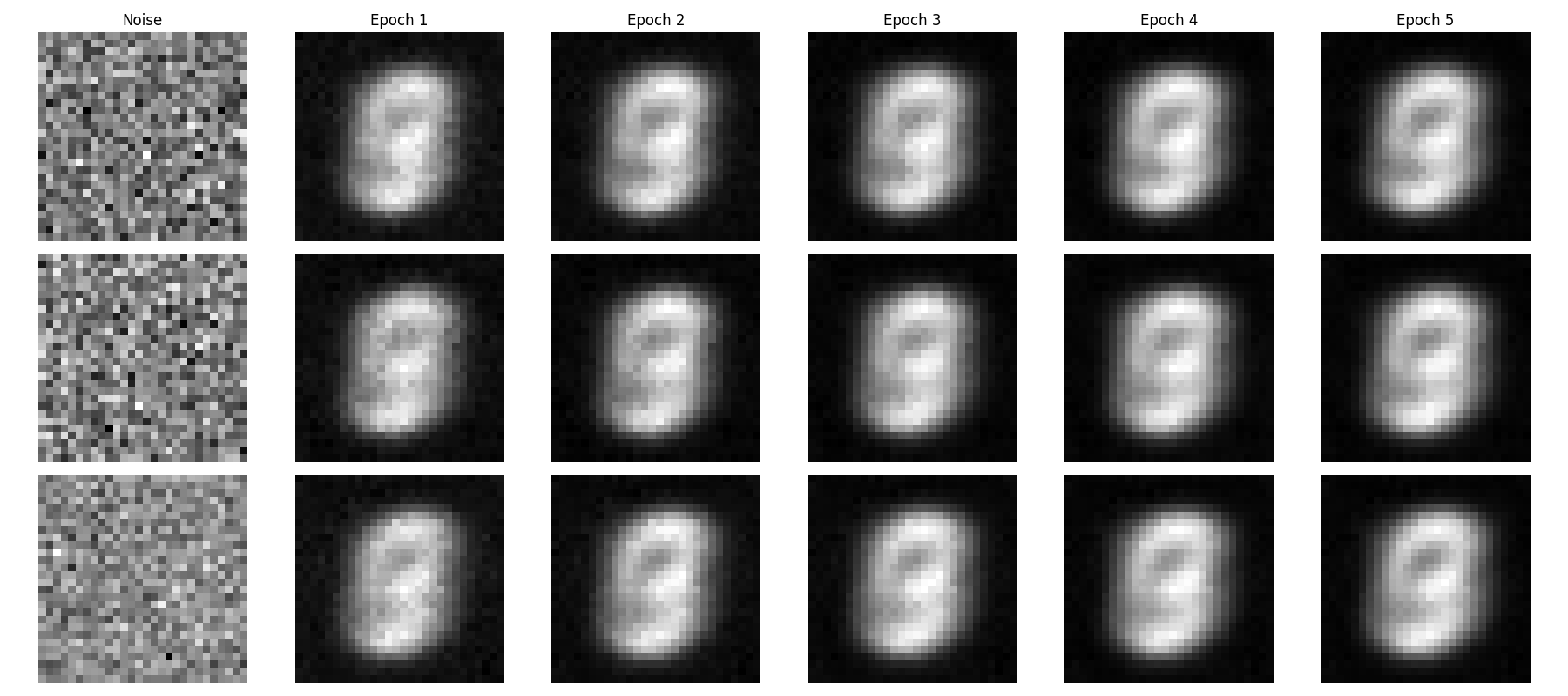
2.1.4 Denoising Pure Noise

The denoiser was further applied to pure Gaussian noise \(z = \epsilon\), \(\epsilon \sim \mathcal{N}(0, \mathbf{I})\), treating generation as a denoising problem with no structured input. The model was trained under the same setup as Section 2.1.2 for 5 epochs, and outputs after the 1st and 5th epoch are shown in Figure 18.

A striking observation is that all generated images are nearly identical, regardless of the noise sample drawn. This can be explained theoretically. Under the MSE loss \(\mathcal{L} = \mathbb{E}_{z,x}[\|D_\theta(z) - x\|^2]\), the optimal denoiser is the conditional expectation:

Since \(Z \sim \mathcal{N}(0, \mathbf{I})\) carries no information about \(X \sim \mathcal{D}_\text{MNIST}\), the two are statistically independent (\(Z \perp X\)), which gives: The optimal denoiser therefore collapses to a constant function: Because MNIST digits are spatially aligned and share a common scale, \(\mathbb{E}[X]\) is a weighted average over all digit classes in which shared structural elements are reinforced, producing the blurred, digit-like image seen in Figure 18.

2.2 The Flow Matching Model

As shown in Section 2.1, one-step denoising does not work well for generative tasks. Instead, flow matching is adopted to iteratively denoise from noise to a clean image. A UNet \(u_\theta(x_t, t)\) is trained to predict the flow — the velocity field guiding noisy samples toward the clean data distribution. In this setup, a pure noise image \(x_0 \sim \mathcal{N}(0, I)\) is gradually transformed into a realistic image \(x_1\).

Intermediate noisy samples are constructed via linear interpolation between the noise \(x_0\) and the clean image \(x_1\):

This defines a vector field describing the position of a point \(x_t\) at time \(t\) as it moves from the noisy distribution \(p_0(x_0)\) toward the clean data distribution \(p_1(x_1)\). For small \(t\), the sample remains close to noise; as \(t\) increases, it approaches the clean distribution.

The flow \(u(x_t, t)\) is the velocity of this vector field — the rate of change of \(x_t\) with respect to time:

A UNet \(u_\theta(x_t, t)\) is trained to approximate this flow, yielding the learning objective:

2.2.1 Adding Time Conditioning to UNet

To condition the UNet on timestep \(t\), a new FCBlock (fully-connected block) operator was introduced to inject the conditioning signal, as shown in Figure 19. Rather than predicting the original image, the model predicts the flow from noisy \(x_0\) to clean \(x_1\), encoding both the image structure and the noise to be removed. Each FCBlock is implemented as Linear(F_in, F_out) via nn.Linear, where F_in = 1 since the conditioning signal \(t\) is a scalar. The pseudo code below shows how \(t\) is embedded and used to modulate intermediate feature maps.

fc1_t = FCBlock(...)
    fc2_t = FCBlock(...)

    # the t passed in here should be normalized to be in the range [0, 1]
    t1 = fc1_t(t)
    t2 = fc2_t(t)

    # Follow diagram to get unflatten.
    # Replace the original unflatten with modulated unflatten.
    unflatten = unflatten * t1
    # Follow diagram to get up1.
    ...
    # Replace the original up1 with modulated up1.
    up1 = up1 * t2
    # Follow diagram to get the output.
    ...

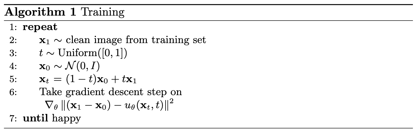
2.2.2 Training the UNet

The time-conditioned UNet \(u_\theta(x_t, t)\) was trained to predict the flow \(x_1 - x_0\) at intermediate timesteps following Algorithm 1 in Figure 20. At each iteration, a clean image \(x_1\) and a timestep \(t \sim U[0,1]\) were randomly sampled, noise \(x_0 \sim \mathcal{N}(0, I)\) was drawn, and the interpolated sample \(x_t\) was computed and fed to the model. The MNIST training set was loaded via torchvision.datasets.MNIST with shuffling enabled and a batch size of 64, with noise applied on-the-fly at each fetch. The UNet from Section 2.2.1 was used with hidden dimension D = 64, with the conditioning signal \(t\) normalized to \([0, 1]\) before injection. The model was optimized with Adam at an initial learning rate of 1e-2, with an exponential decay scheduler \(\gamma = 0.1^{(1.0/\text{num\_epochs})}\) applied after each epoch via torch.optim.lr_scheduler.ExponentialLR(...). 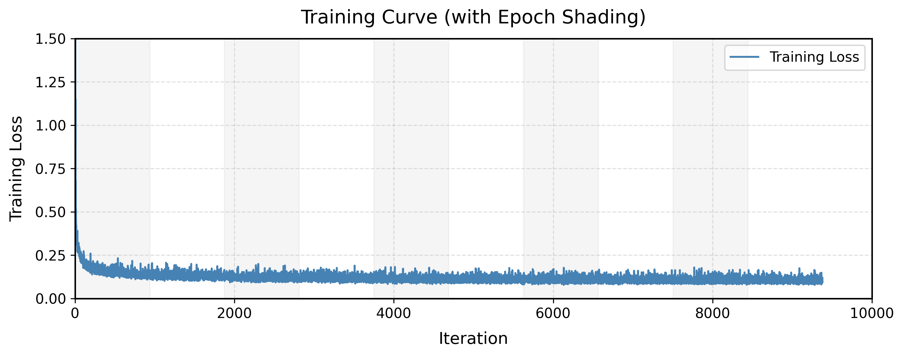Figure 21 shows the training loss curve, indicating rapid convergence within the first 100 iterations; beyond that, the loss continues to decrease but at a much slower rate. The model improvement from epoch 2 to epoch 10 is marginal.

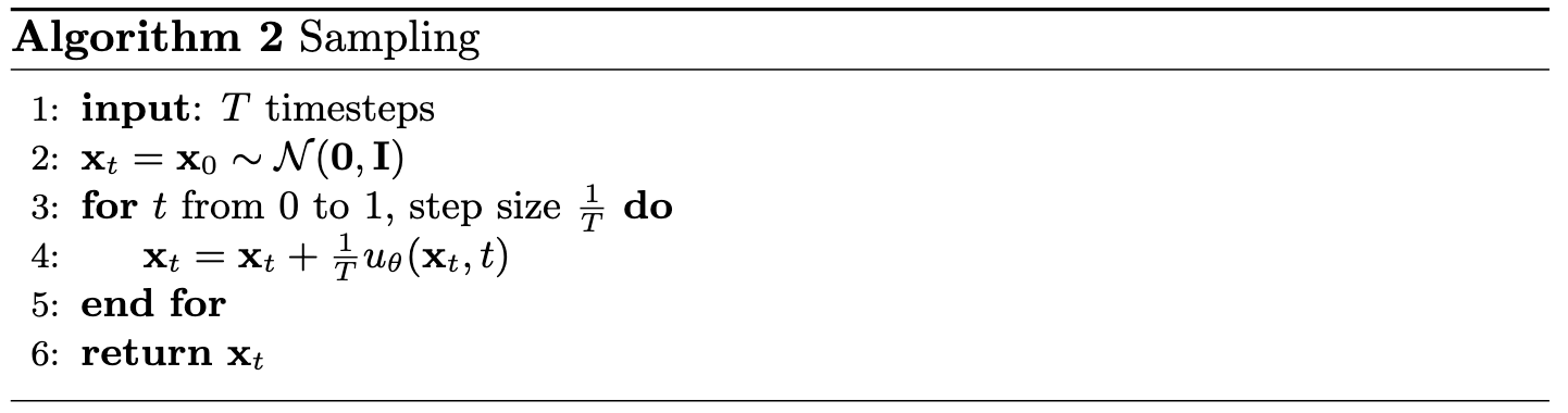
2.2.3 Image Sampling

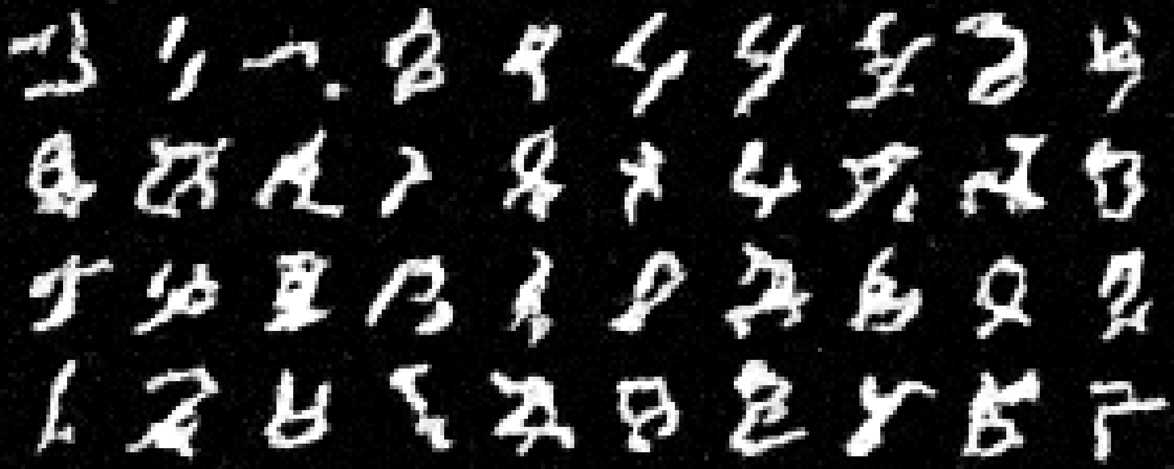
Once trained, the time-conditioned UNet was used to generate images by iteratively denoising pure Gaussian noise. The sampling procedure follows Algorithm 2 (Figure 22), which applies a simple Euler method with a fixed step size of \(1/T\) over \(T = 50\) steps. Figure 23 shows generated samples at epochs 1, 5, and 10. The model progressively learns to produce more realistic and diverse digits as training advances. While some visual artifacts persist, the results are substantially more coherent than those from the one-step denoiser.

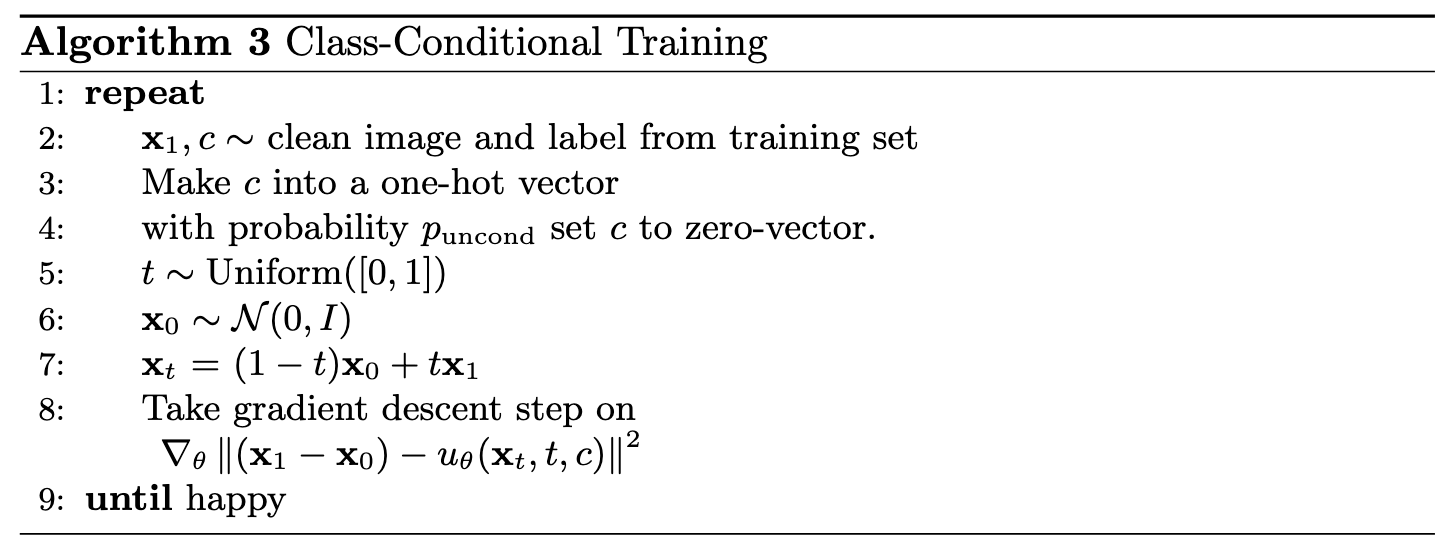
2.3 Class-Conditioned Flow Matching

To improve denoising quality and enable explicit control over the output, the UNet was further conditioned on the digit class (0–9) in addition to the timestep \(t\). This required adding two more FCBlocks to inject the class signal \(c\), represented as a one-hot vector rather than a scalar. To retain unconditional generation capability — analogous to classifier-free guidance in Part 1 — dropout was applied to the class conditioning: with probability \(p_\text{uncond} = 0.1\), the class vector \(c\) was set to zero during training, allowing the model \(u_\theta(x_t, t, c)\) to operate without class information. The pseudo code below shows how both \(t\) and \(c\) are embedded and used to modulate the intermediate feature maps:

fc1_t = FCBlock(...)
    fc1_c = FCBlock(...)
    fc2_t = FCBlock(...)
    fc2_c = FCBlock(...)

    t1 = fc1_t(t)
    c1 = fc1_c(c)
    t2 = fc2_t(t)
    c2 = fc2_c(c)

    # Follow diagram to get unflatten.
    # Replace the original unflatten with modulated unflatten.
    unflatten = c1 * unflatten + t1
    # Follow diagram to get up1.
    ...
    # Replace the original up1 with modulated up1.
    up1 = c2 * up1 + t2
    # Follow diagram to get the output.
...

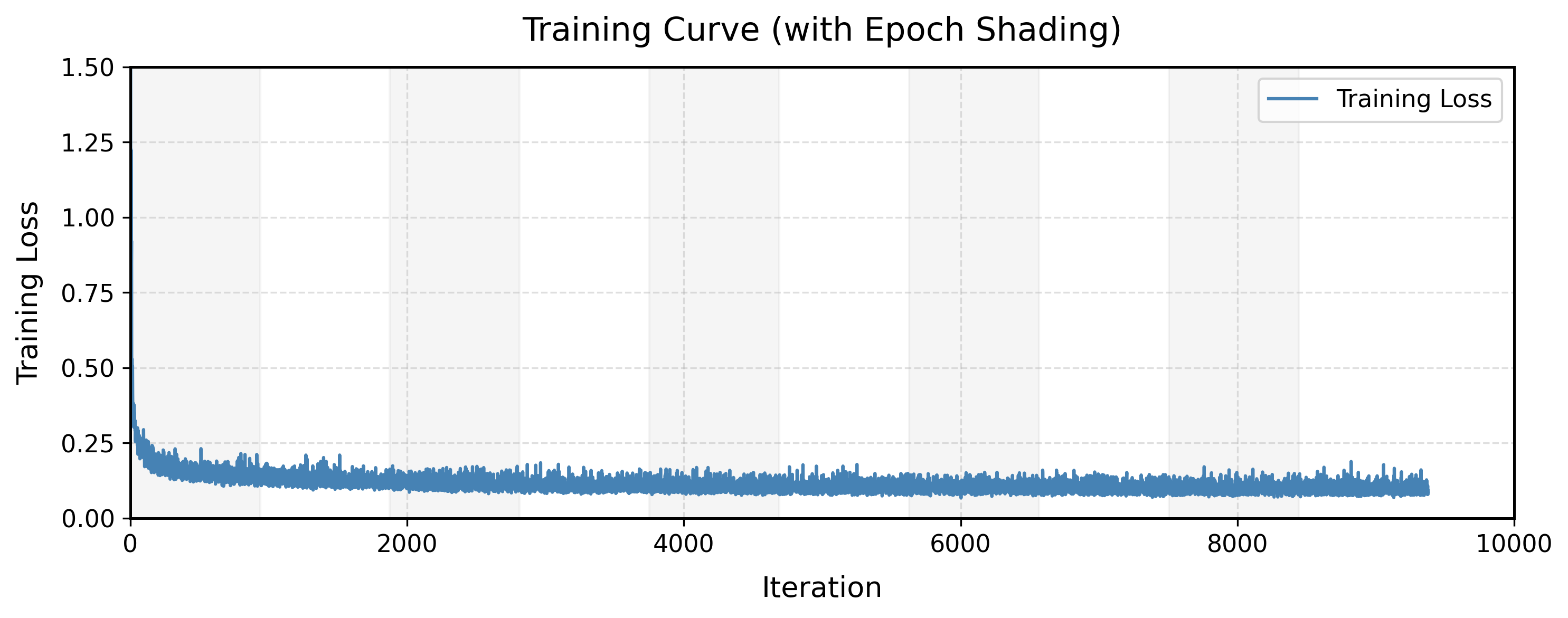
2.3.1 Training the Class-Conditioned UNet

Training the class-conditioned UNet followed the same procedure as the time-conditioned model in Section 2.2.2, with one key addition: the class conditioning vector \(c\) was injected alongside \(t\), and unconditional generation was applied periodically by zeroing out \(c\) with probability \(p_\text{uncond} = 0.1\), following Algorithm 3 (Figure 24). The resulting training loss curve is shown in Figure 25.

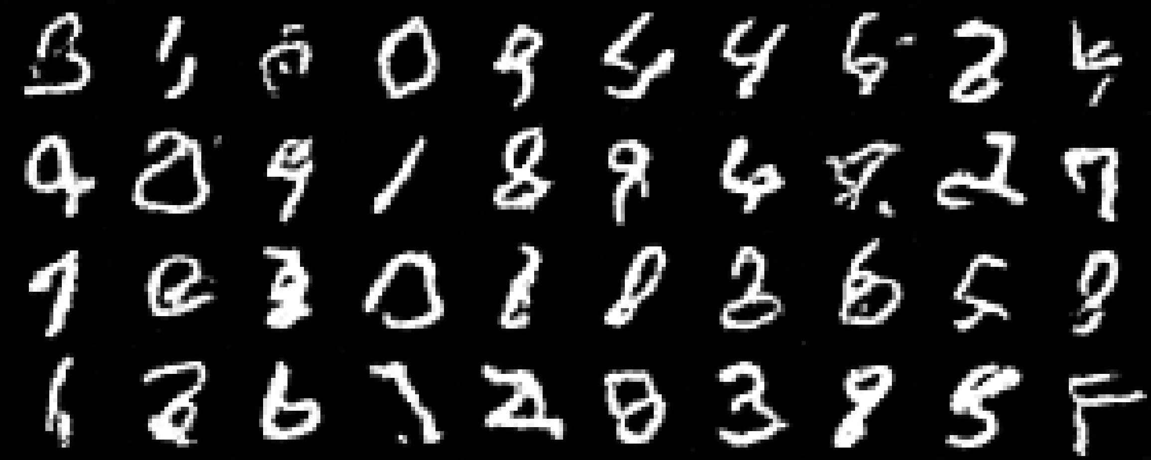
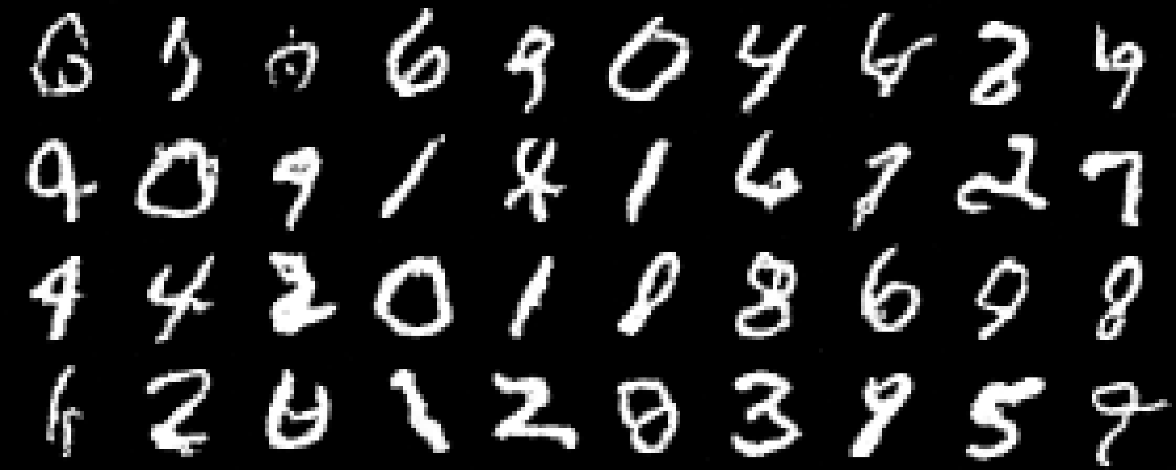
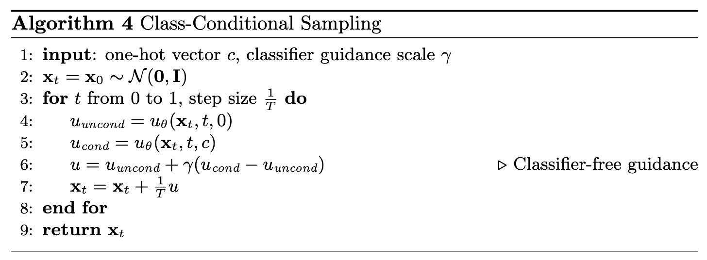
2.3.2 Sampling from the Class-Conditioned UNet

The class-conditioned model was used to generate images via classifier-free guidance (CFG), following Algorithm 4 (Figure 26). A guidance scale of \(\gamma = 5.0\) was applied during sampling to steer the outputs toward the target class and enhance overall generation quality.

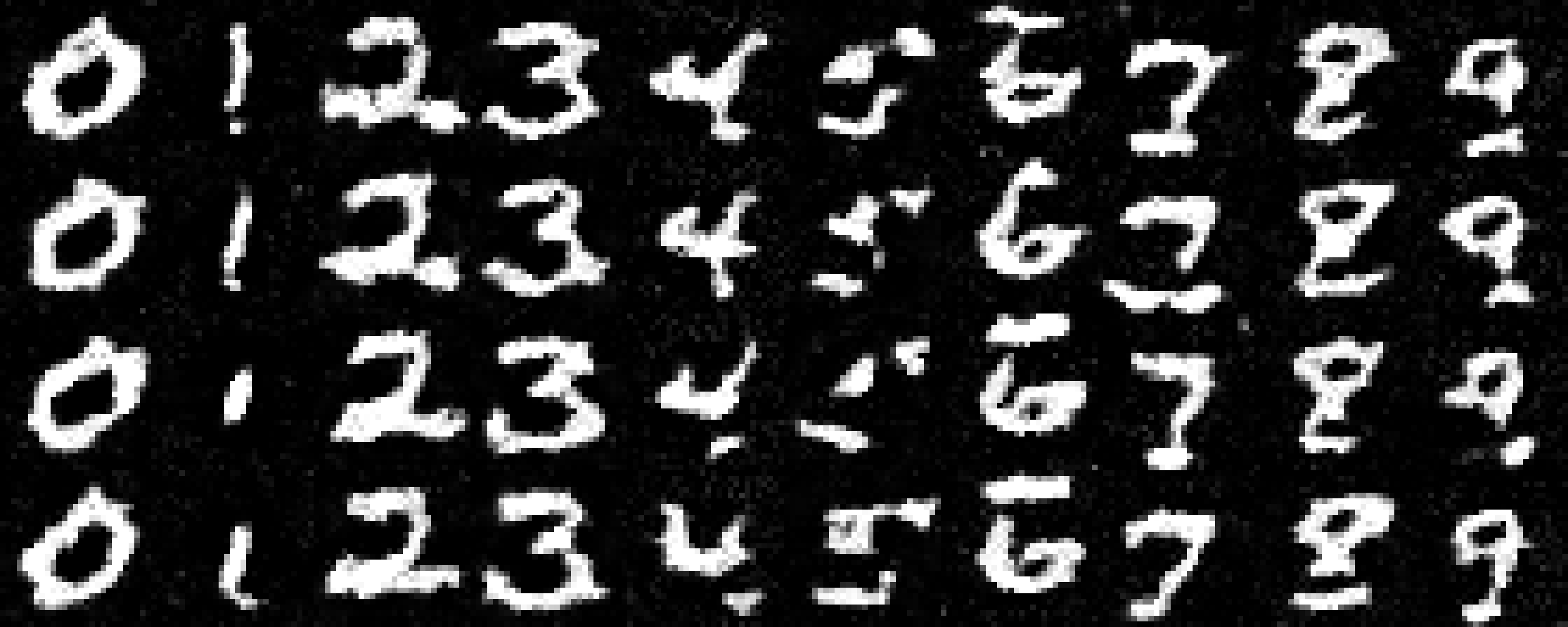
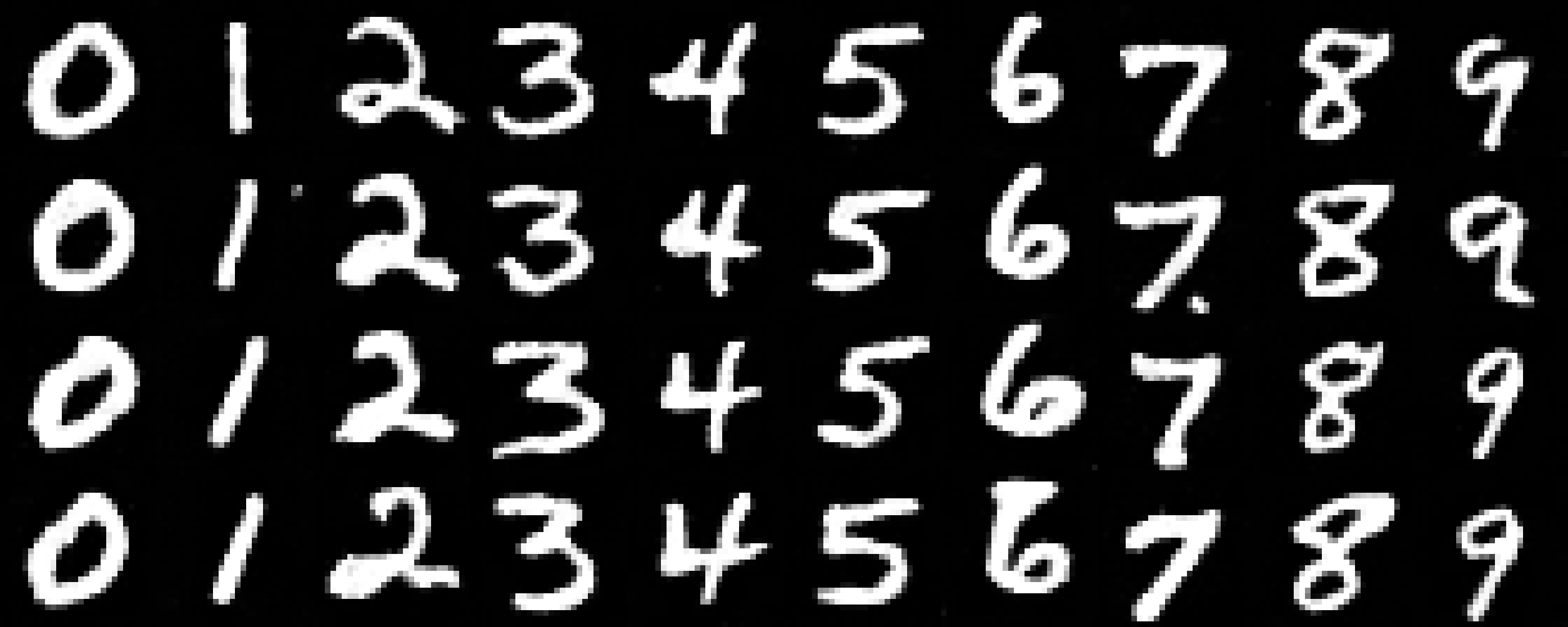
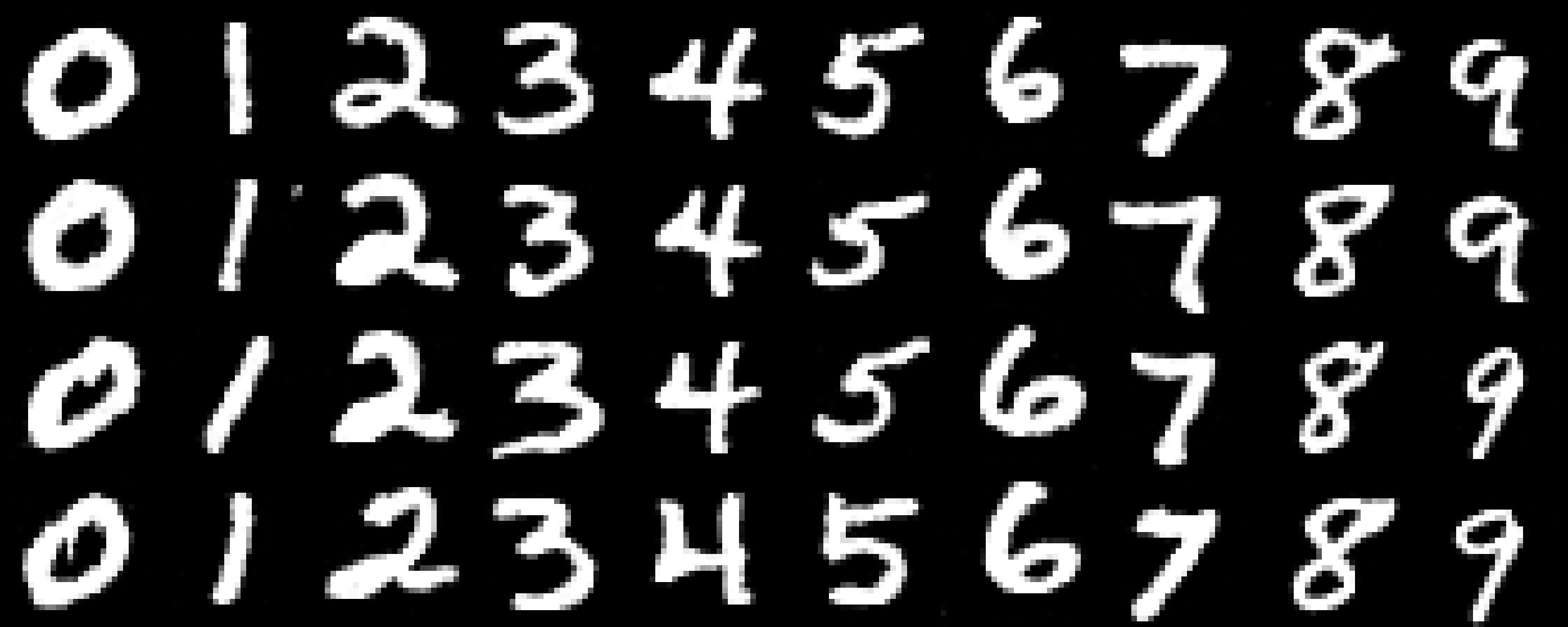
Figure 27 shows generated samples at epochs 1, 5, and 10. The class-conditioned model with CFG produces noticeably sharper and more recognizable digits compared to the time-conditioned model alone, confirming the benefit of explicit class conditioning for generation quality.

References

- Ho et al., Denoising Diffusion Probabilistic Models, NeurIPS 2020. [arXiv]
- Saharia et al., Photorealistic Text-to-Image Diffusion Models with Deep Language Understanding, NeurIPS 2022. [arXiv]
- Song et al., Denoising Diffusion Implicit Models, ICLR 2021. [arXiv]
- Ho & Salimans, Classifier-Free Diffusion Guidance, NeurIPS Workshop 2021. [arXiv]
- Meng et al., SDEdit: Guided Image Synthesis and Editing with Stochastic Differential Equations, ICLR 2022. [arXiv]
- Lugmayr et al., RePaint: Inpainting using Denoising Diffusion Probabilistic Models, CVPR 2022. [arXiv]
- Geng et al., Visual Anagrams: Generating Multi-View Optical Illusions with Diffusion Models, CVPR 2024. [arXiv]
- Lipman et al., Flow Matching for Generative Modeling, ICLR 2023. [arXiv]